Top 8

Network graph made out of thread wrapped around screws on a poster board.

Given the “agnostic” nature of our chosen dataset, I felt a certain level of freedom to explore what the process would be to generate a physicalized network graph versus pursuing a “normal” data analysis with a visual approach.  Here I started the process with a firm framework of the project’s materials (string, nails/screws/ mounting board), mode of output (network graph), and other sensing modalities (tactility and aurality). The data would be secondary to the process of making a physical artifact. Did I just intentionally open the “bias door” with my predetermined framework? More on that later…

The resulting physical artifact in this case would be a data physicalization “whose geometry or material properties encode data” (Jansen et al., 2015). What is it not? It would not be a scale model, architecture model or a figurative sculpture (Dragicevic et al., 2021). Data physicalization does align and sometimes intersect with other areas of research within the human computer interaction realm, like visualizations (of course) – which utilize computers to process “abstract” data into visual representations for easier relatability and understanding. Another area, tangible interaction, focuses on the interactive systems that hinge on physical artifacts as the vehicle to both represent and control “computational media” (2021). It is interesting to note that the visual facet of these other data representation modalities never fully divorce from their definition or explanation. Notably, “Design Principles for Visual Communications” by Agrawala et al., 2011 is referenced multiple times to frame the process of transforming abstract data to a human consumable format via “the three-stage methodology [that] involves first identifying physical characteristics to be incorporated into the design, followed by instantiation of those characteristics, then evaluation of the physical characteristics”(Drogemuller et al., 2019). The sense of sight is front and center in the world of data science and arguably in Digital Humanities as well.

But we have other senses and for some, a limitation on what others assume as the default sense.  Data physicalization focuses on “data-driven tasks, such as data exploration and data communication”(Dragicevic et al., 2021), which opens the door to increased pathways for abstract data constructs to connect to human understanding. Jansen et al. posit “all senses can participate in information gathering and they each have unique characteristics that can be leveraged by physicalizations”(Jansen et al., 2015). 

As the field has developed in this area, the term “data visceralization” entered into the lexicon thanks to Kelly Dobson in the early 2000s, and “later popularized by Luke Stark”(Wernimont, 2022). Defined as the “representations of information [that] rely on multiple senses including touch, smell, and even taste, [that] work together to stimulate our feelings as well as our thoughts”(Stark, 2014),  it has become more prevalent in the discussion and research. There is an interesting nuance that Stark additionally points out in that “visceral data has the potential to level out our reactions the opposite way [from a solely visual consumption of information]: as well as appreciating a problem or issue rationally, users prompted to engage viscerally will have a well-rounded sense of their own intellectual, emotional and physical stance on the matter at hand”(2104).

To arrive at the point of “visceralization” and/or “physicalization” in my own project, lengthy and laborious efforts were required to prepare the data. First I identified the key columns of data that would best suit an output of a network graph. I initially chose: “Unique Identifier”, Episode_ref ,track_name, date, castaway_ref , std_artist, and std_name from the “disk” dataset.   Partly by design, I chose those same columns during the labor intensive encoding error and “missing-ness” identification process Ava, Carol, Lubov, and I performed for the Map & Key. From that point I continued to work with the data in OpenRefine to combine like values through text facets, algorithmic clustering, to remove special characters, and perform visual checks in preparation for the physical output. Essentially I made decisions about what data would stay, be “fixed”, or disregarded.

Another decision point arose with the representation of the data as nodes or edges. I applied a Python script to create the nodes pair and the connecting edges with weight (= occurrences). Here is when the process deteriorated (or perhaps more kindly, iterated through on repeat). Multiple trial attempts of identifying the nodes and edge relations for the final output transpired. Initially I considered the entire “disk” dataset, but that was not a realistic choice as it was too large to transfer with the materials ( or time) I had available. I processed a version where I broke down the episodes by decades (compare 60s vs 00s, eg). From there I iterated through a couple more choices of how to splice the data: song choice as node with the artist as edge, then castaway as node and artist as edge, then the artist as nodes castaways (guests) as edges – their co-occurrence choice. I even attempted to pull a subset of the data with a randomizer (1 choice per year to process using the artists as the nodes and the episode date as the edge, decades). The final attempt, Trial 6, resulted in the selection of the top 8 artist choices (nodes) across all the years two of those top choices co-occurred(edges).

The resulting nodes and edges files were imported into Gephi, an open graph visualization software. I used Gephi to visualize the nodes and edges table to iron out preliminary layout and  run some statistics on degree and modularity. I played around with the layout (color, size, ranking) in preparation for the physicalization build.

Physicalization of the Absence

The resulting data subset I arrived at included only 4478 artist choices for the top 8, leaving 21,782 choices not “used”.  That’s quite a bit of data not used!  I was reminded about an article Cat Hicks published on Data Science by Design where they talk about what is left behind when processing data for an intended outcome, “Sometimes I like to call this ‘when we miss missingness,’ a quip to remind myself that we need to understand data not just in terms of datasets but in terms of the context around it. We need to ask what data was collected and, perhaps more importantly, what data was left out”(Hicks, 2022). Which is why I chose to bring them into the fold and highlight their presence through another tactile mode.

With pen and paper, I created a series of dots that each represented 2 choices each, total of 10,891. I would later affix these textural dot papers to the underneath of the physical network to symbolize that the data doesn’t cease to exist when choices are made to exclude, parse, and foreground visualized data.

Sonification of Labels /Materialization of Connections

The physical network graph assembly involved screwing in screws into the foam core board which served as the nodes that the edges would connect to via crochet thread in various colors representing the top 8 artist choices. The Python nodes and edge table was my instruction list for the wrapping which colored thread (edges) between 2 screws (nodes).  The weight (occurrences) was the amount of thread loops connecting the screws (one thread thickness = 2 occurrences). The nodes’ label was supplied by a miniature recording device with the recorded name of the top artist playing when a button was pressed.

Technical Process

The technical process for my individual visceralization built upon the initial encoding error identification processing of the Map & Key. I provide detail to both steps below.

Group Map & Key – Data Processing

  • Divided the data between “discs” and “castaways” sheets amongst Ava, Carol, Lubov, and myself to determine the “Grey, Black, and White” of the data. Grey = data has issue, black= data has no issue, white= data is absent
    • Columns I reviewed:
      • Sheet: discs
      • Columns: (blank), track_name, trackNo, date, std_artist, std_disc, Std_name
  •  JD – DID_discs files collected the criteria of what processes were run/ performed to identify the “grey and white”
    • Exported JSON files from Open Refine post processing through different clustering methods (+ merge)
    • Openrefine>Cluster and edit>Method:Key Collision>Keying Function:Fingerprint
    • Openrefine>Cluster and edit>Method:Key Collision>Keying Function: ngram-fingerprint2
  • Manually collected lists with reasoning on why those values should be “grey”
    • The same name appearing with different spelling, spaces, capitalizations
      • Most of the clustering took care of those anomalies
      • Visual check completed to see if anything remains
    • Issue with classical music in std_disc values appeared.
      • Inconsistencies with format, naming conventions, inclusion of or absence of suite no’s, key, op no’s, movement
      • In order to review and compare these values, applied text filters in OpenRefine and filtered on text strings that are typically found in “classical” music titles. (not case sensitive filter)
        • “concerto” (282)
        • Tried “minor” (335 values)  and major” (400 values)
          • Saw repeats after identified “concerto”
          • Due to similar issues with track_name and sheer volume needed to review visually, for consistency’s sake, only did a visual pass with “concerto” filter
    • Issue with classical music in track_name values appeared.
      • In order to review and compare these values, applied text filter in Open Refine and filtered on text strings that are typically found in “classical” music titles.
        • “Concerto” (417)
        • Tried “minor” (613 values)  and major” (705 values)
  • Provided exported OpenRefine clustering results via JSON to my teammate Lubov where she processed into indexes for Map & Key production.

Individual Data Processing

  • Exported just the “discs” sheet from Desert Island Disks and removed the unneeded fields. The following fields remained: Unique Identifier, episode_ref, track_name, date, castaway_ref, std_artist, std_name
  • In OpenRefine iterated through the following checks to see if they were  present in the data. The difference at this point from what was performed when processing the data for the Map & Key is actually reconciling and updating the data with values that make sense semantically → {{DISCS_desert_island_discs_OnlyNeededFields}}
  • Special Characters (find and replace with source language characters) for:
    • track_name (19 that couldn’t replace)
    • std_artist
    • std_name
  • Blanks?
    • track_name (none)
    • std_artist (15 – these correspond to some  the 19 rows that couldn’t replace special characters)
    • std_name (none)
    • date(none)
  • Cluster and Merge
    • track_name
      • Openrefine>Cluster and edit>Method:Key Collision>Keying Function:Fingerprint (select all)
      • Openrefine>Cluster and edit>Method:Key Collision>Keying Function: ngram-fingerprint2 (select all)
      • Openrefine>Cluster and edit>Method:Key Collision>Keying Function: Beider-Morse
        • Only select clusters
        • As seen below, many of the clustering suggestions were related, but were different acts, variations, scenes, etc.
Example of one of the clustering algorithms used in OpenRefine
  • Std_artist
    • Openrefine>Cluster and edit>Method:Key Collision>Keying Function:Fingerprint (select all)
    • Openrefine>Cluster and edit>Method:Key Collision>Keying Function: ngram-fingerprint2 (select all)
    • Openrefine>Cluster and edit>Method:Key Collision>Keying Function: Beider-Morse
      • Only one selected cluster grouping 
    • Manually combine some classical composers, like “peter” into “pyotr” & “mozart” to his full name
  • Std_name
    • Openrefine>Cluster and edit>Method:Key Collision>Keying Function:Fingerprint (select all)
    • Openrefine>Cluster and edit>Method:Key Collision>Keying Function: ngram-fingerprint2 (select all)
    • Openrefine>Cluster and edit>Method:Key Collision>Keying Function: Beider-Morse
      • Only one selected cluster grouping 
Notes about the Data:
  • Std_artist:
    • Noticed that the name of the song is sometimes listed as the artist
      • Ex: violin concerto no 2
      • Did not change or edit this scenario

Code + files for the “trials” found here.

TRIAL 1: 

  • Used the whole dataset to make the first pass at creating the nodes and list: it took a VERY long time. (4+ hours, but I aborted the script before it ever completed)
  • Consideration to compare 2 decades at a time (eg 1950’s to 2010’s)
  • Compare 1 vs Compare 2 (1980’s doesn’t have a decade to compare to, run against itself?)
    • In the data, I created a column called “Decade” and assigned values of “40s” when date = 1940-1949, “50s” when date = 1950-1959 , etc. These values were assigned accordingly: 40s, 50s, 60s, 70s, 80s, 90s, 00, 10s, 20s

Compare 1

Compare 2

1940’s + 1950’s = 3738 choices

2020’s + 2010’s = 3528 choices

1960’s = 4201 choices

2000’s = 3187 choices

1970’s = 4095 choices

1990’s = 3242 choices


1980’s = 3647 choices


TRIAL 2: 

  • Ran .py script to make 40-50vs10-20 & 60vs00
  • Noticed that the source and target were the same:

  • Hypothesis on why: because using the castaway_ref as the node, these aren’t unique due to the repeat of 8 choices the castaways (std_name) make per episode. Need to identify a way to have a unique identifier as the node

TRIAL 3: 

  • Possible solution: create a unique identifier for each episode that accounts for the dimension of the decade and the shared choice of the artist will be the edge connecting them (had to sacrifice the std_name / castaway label for the sake of uniqueness)
  • Assign consecutive numbers to the “decade” data when the “date” column is sorted oldest to newest, example:

date

decade_episode

1/4/1960

60-1

1/4/1960

60-2

1/4/1960

60-3

1/4/1960

60-4

1/4/1960

60-5

1/4/1960

60-6

1/4/1960

60-7

1/4/1960

60-8

1/11/1960

60-9

1/11/1960

60-10

1/11/1960

60-11

1/11/1960

60-12

  • “Decade_episode” ID will now serve as the unique identifier. Might have to use this as a the label too (nothing unique to make identifier)
  • For the “label” of “Decade_episode” ID, joined the “Decade_episode” with the “std_name”:
    • =JOIN(“-“,E25439,I25439)
    • 20-444-robert macfarlane

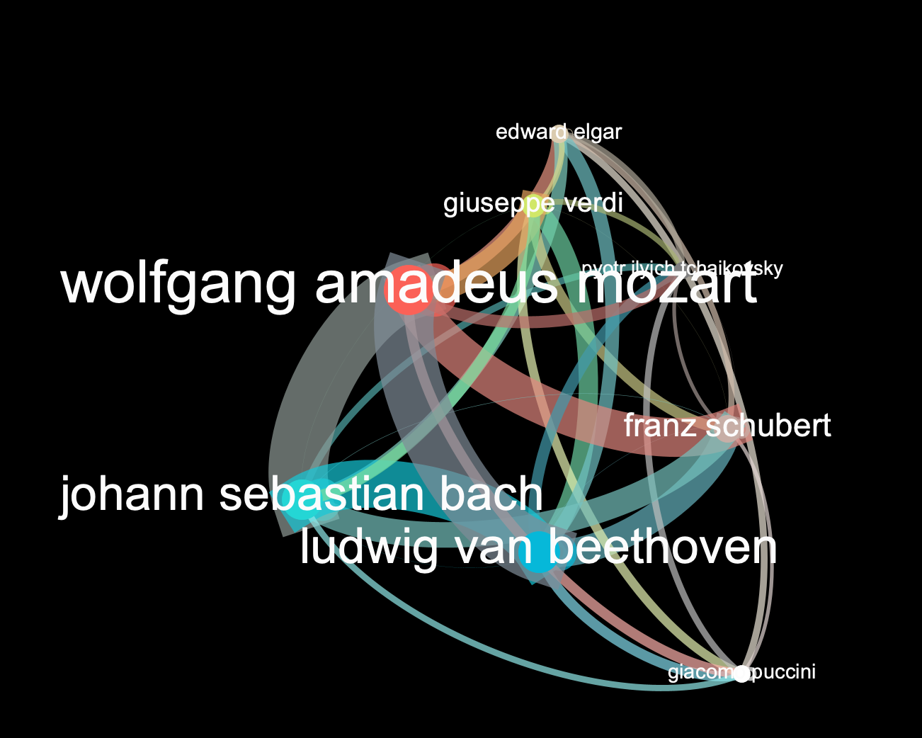
Reflection about nodes and edges formation:

  • What are the shared artist (std_artist) choices between 2 castaways (std_name)
    Explanation of activity between the nodes(TRIAL 1 & 2):
  • For (std_artist)  A, they were selected as an artist of a desert island disc by castaway  1 and castaway 2. No other artists followed that pattern. The weight of “1” reflects that singularity of occurrence. However, castaway 1 and castaway 4, both selected (std_artist)  C. The weight reflects that shared occurrence by the number “2”. 

Source castaway

Target castaway

Shared Artist Choice

Weight

std_name 1

std_name 2

std_artist A

1

std_name 1

std_name 3

std_artist B

1

std_name 1

std_name 4

std_artist C

2

  • Need to decide:  The nodes = std_artist or nodes = castaway_ref

TRIAL 3B:

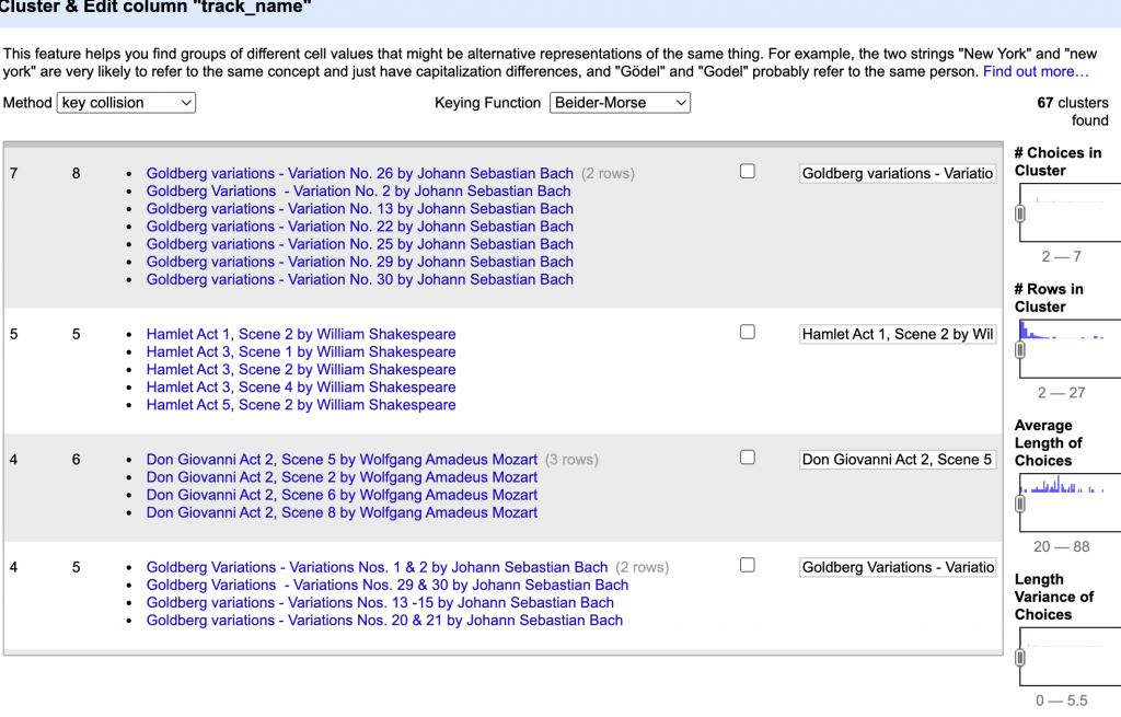
    • Co-occurrences of an artist within a decade

Source episode choice

Target episode choice

Artist

Weight

40-111

40-216

std_artist A

1

40-111

10-782

std_artist B

1

40-111

20-186

std_artist C

1

  • The blanks: total of 15 for std_artist, but they have track_name values. See below:
  •  Can that be incorporated into the network graph (the absence)? Maybe this can be made manually, through the process of creating a network graph of the absence?

track_name

To Feggaraki by Αλίκη Βουγιουκλάκη

The Boys of Piraeus from Never on Sunday by Μελίνα Μερκούρη

Song Of The Volga Boatmen by –§—ë–¥–æ—Ä –®–∞–ª—è–ø–∏–Ω

Compline Isiah’s prophecy, Znamemy Chant by –ê–ª–µ–∫—Å–∞–Ω–¥—Ä –î–º–∏—Ç—Ä–∏–µ–≤–∏—á –ö–∞—Å—Ç–∞–ª—å—Å–∫–∏–π

Evening by Τίτος Καργιωτάκης

Slowly Slowly by Λόλα Τσακίρη

Glory To Thee Oh Lord (from Twofold Litany) by –§—ë–¥–æ—Ä –®–∞–ª—è–ø–∏–Ω

Allegro Bouzouki by Γιώργος Ζαμπέτας

Down the Petersky by –§—ë–¥–æ—Ä –®–∞–ª—è–ø–∏–Ω

The Miller’s Aria (from The Rusalka) by –§—ë–¥–æ—Ä –®–∞–ª—è–ø–∏–Ω

Down the Petersky by –§—ë–¥–æ—Ä –®–∞–ª—è–ø–∏–Ω

Glory To Thee Oh Lord (from Twofold Litany) by –§—ë–¥–æ—Ä –®–∞–ª—è–ø–∏–Ω

Glory To Thee Oh Lord (from Twofold Litany) by –§—ë–¥–æ—Ä –®–∞–ª—è–ø–∏–Ω

Song Of The Flea by –§—ë–¥–æ—Ä –®–∞–ª—è–ø–∏–Ω

Mort De Don Quixote by –§—ë–¥–æ—Ä –®–∞–ª—è–ø–∏–Ω

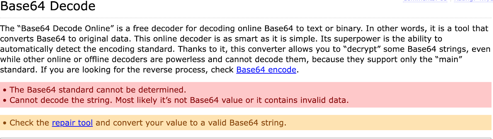
  • Tied to run the track_name  through base64 decoder, (As suggested by teammate Lubov), but none of the encoding was recognizable:
  • Since moving to Trial 4, it was not necessary to reconcile these values as they were not randomly selected.

TRIAL 4:


Source Artist

Target Artist

Castaway Ref

Weight

std_artist A

std_artist B

2967

1

std_artist A

std_artist C

1291

1

std_artist A

std_artist D

807

1

  • Couldn’t get this to populate an edge table… it was just blank if I use artist as the node.
  • Need to Re-do

Source castaway

Target castaway

std_artist_id

Weight

928

1191

art-6

1

2953

649

art-17

1

928

54

art-19

1

  • Selecting only 1 artist choice from each year
    • Since not all the months/ dates/ or even years are present, selecting a single month- date across all the years represented in the data set was impossible (i.e. the same month-date).
    • Some consideration was given to the possibility of selecting a month/day/year artist choice representation based:  a monthly range or highest yield of choices on a particular month-day.
      • This doesn’t result in a solution that would represent every month or every year
  • New Criteria = use a randomizer tool to select an artist choice for every year. Used: https://www.gigacalculator.com/randomizers/random-picker.php

TRIAL 5:

  • Noticed that the data file base I was using didn’t have the same total # for rows; DISCS-desert-island-discs-OnlyNeededFields_OpenRefined 25,459 vs 26260_DISCS-desert-island-discs-OnlyNeededFields 26,259
    • Pivoted to the file with the higher amount of rows
  • Made artist ID’s for all the artists in the whole dataset.
  • Selected just the 80’s decade to try using the new artist ID’s (as the nodes) with date as the edge
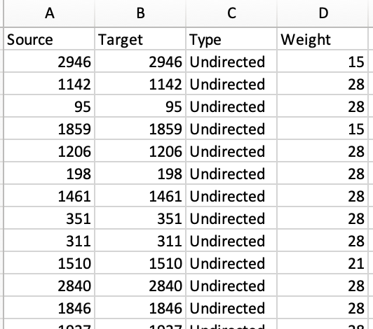
  • Successful run of .py  (made a weighted adjacency table)
  • When I loaded it into Gephi, I got an error of duplicate nodes ( maybe due to pulling in the date they were mentioned as a choice?). I removed duplicates just on the vertices file and was accepted into Gephi without errors

TRIAL 4B: 

  • Moved back to a previous data processing iteration (Trial 4) and tried using the randomized selection to process using the artists as the nodes and the episode date as the edge.
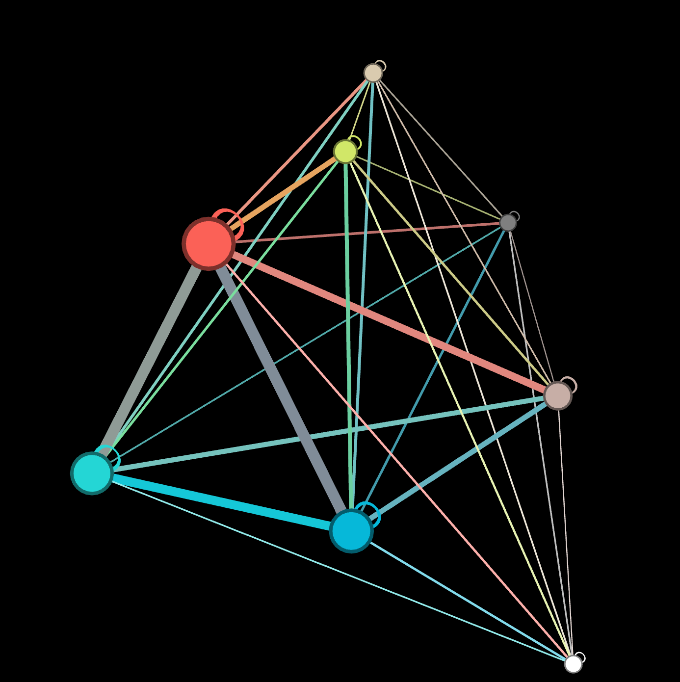
    • The edge list resulted in an incomplete nodes/edges list, shown below. Decided to abandon the randomized tactic.


TRIAL 6: 

After much consideration and reflection with the different iterations of data processing trials, I desired to have the network graph represent something of substance of the dataset while still maintaining the ability to execute it with the materials and time available.

Top 8 artist choices (nodes) across all the years those choices were made (edges) 26260_DISCS-desert-island-discs-OnlyNeededFields sheet as the main starting point.

  • Noticed extra grouping that needed to take place in order to consolidate like values (e.g. bach to johann sebastian bach , name of song by beethoven to ludwig van beethoven, schubert to  franz schubert, etc.)
    • Updated the corresponding “std_artist_id” accordingly (to match main std_artist_id)

Final top 8:


std_artist

std_artist_id

Total occurrences

wolfgang amadeus mozart

A5418

999

ludwig van beethoven

A3004

841

johann sebastian bach

A2427

812

franz schubert

A1618

413

giuseppe verdi

A1815

373

edward elgar

A1326

350

pyotr ilyich tchaikovsky

A3932

345

giacomo puccini

A1790

345


Python script for nodes and edges table and final output here.

The total amount of rows for this iteration = 4478

After processing the data, I loaded in the nodes and edges table to create a primary network visualization in Gephi as a guide. I applied various algorithms, statistics, and assigned color and size to those results. 
The output of this process served as my guide for the network graph physicalization.

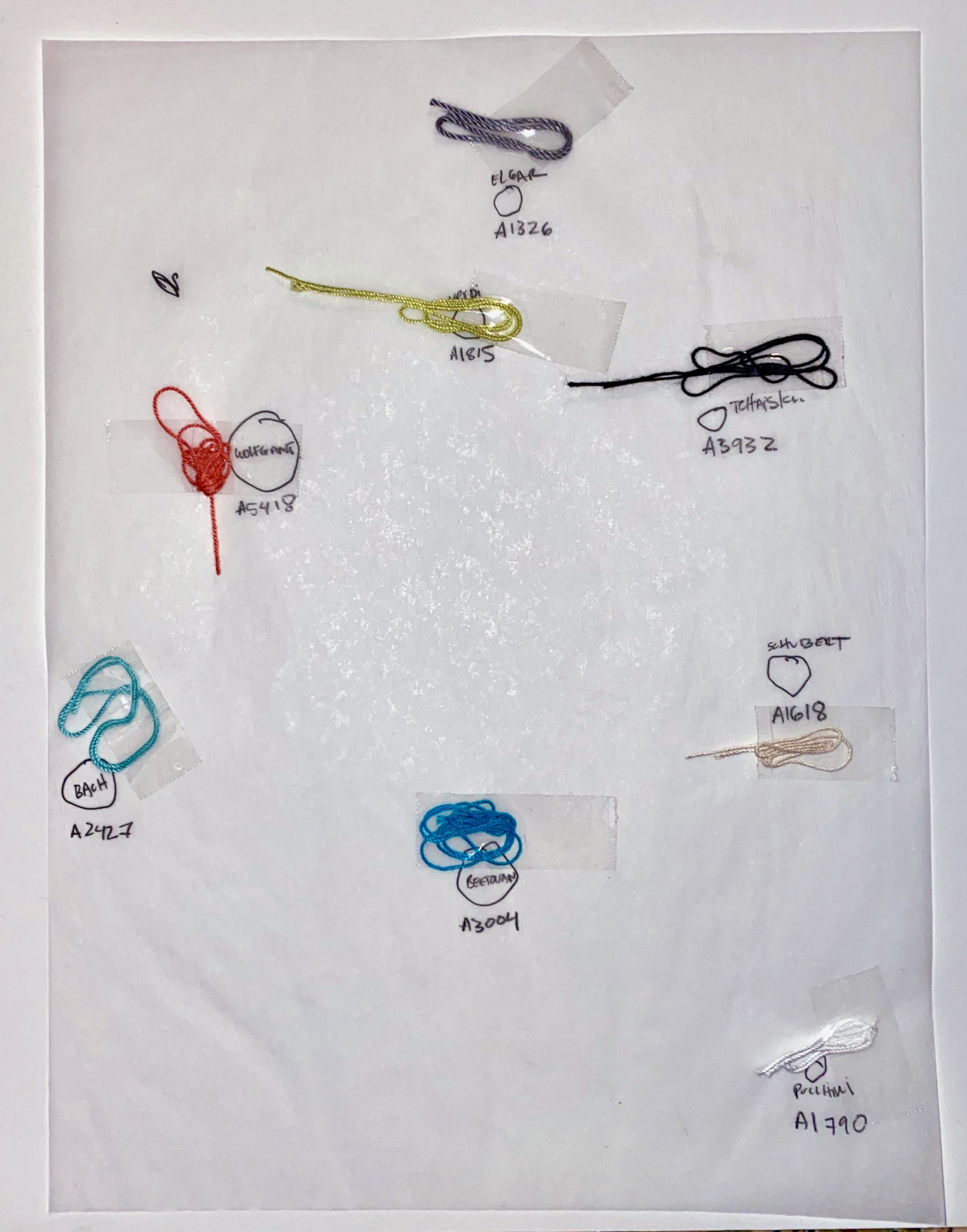
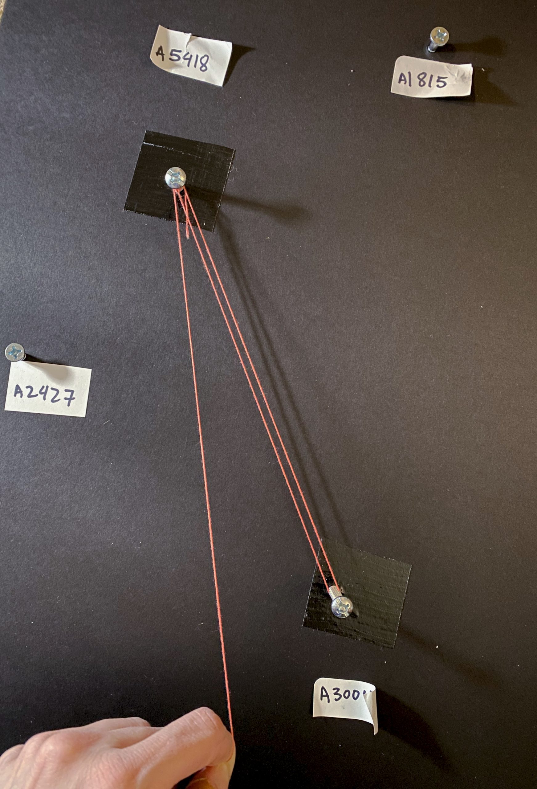
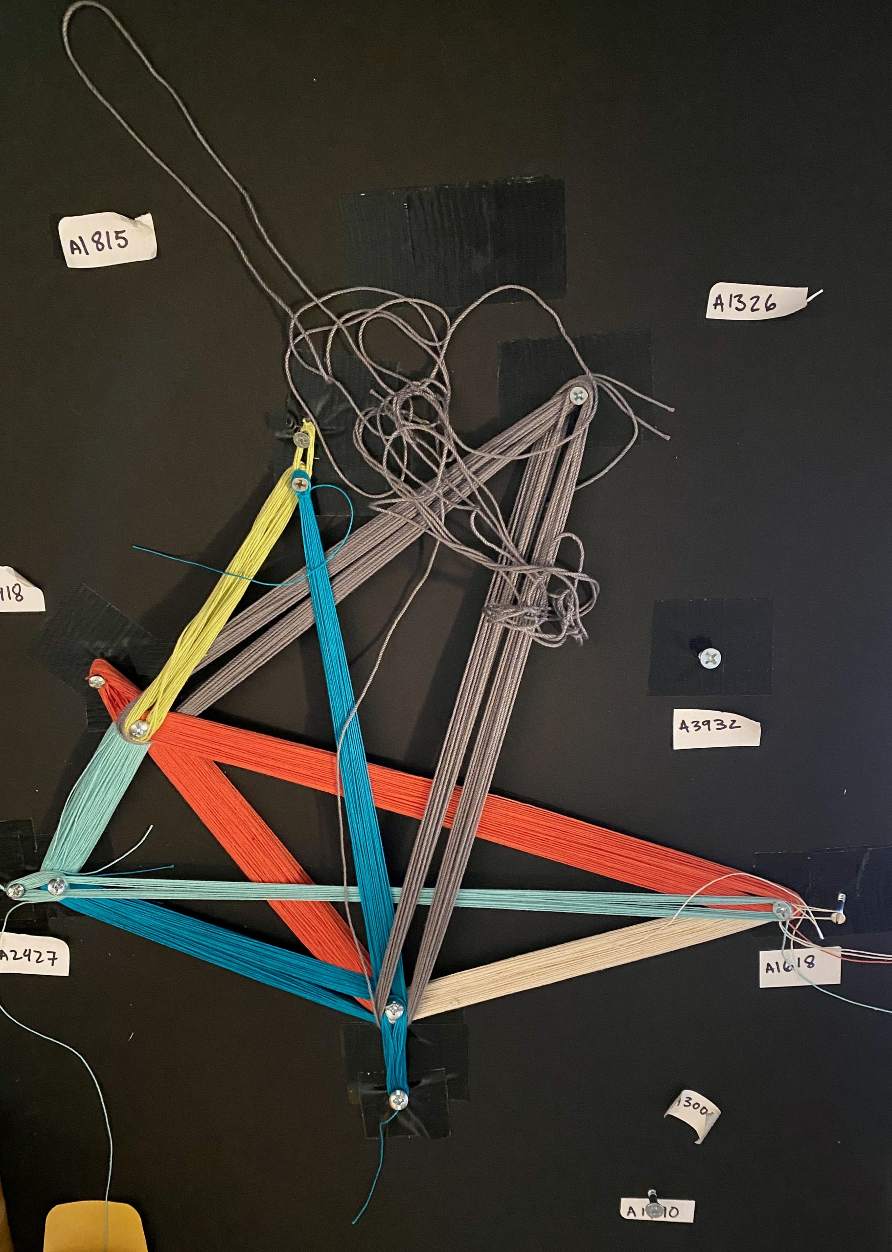
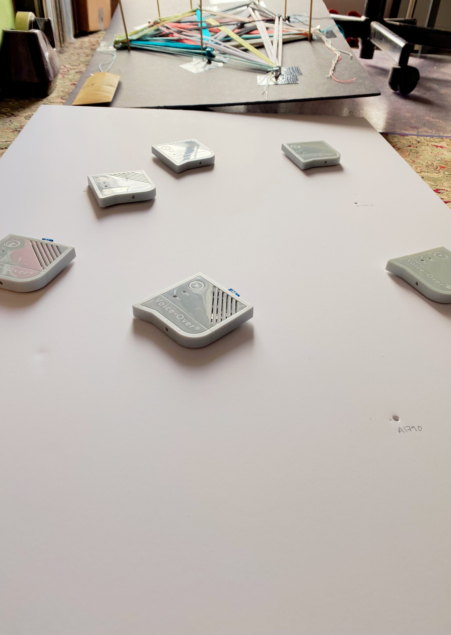
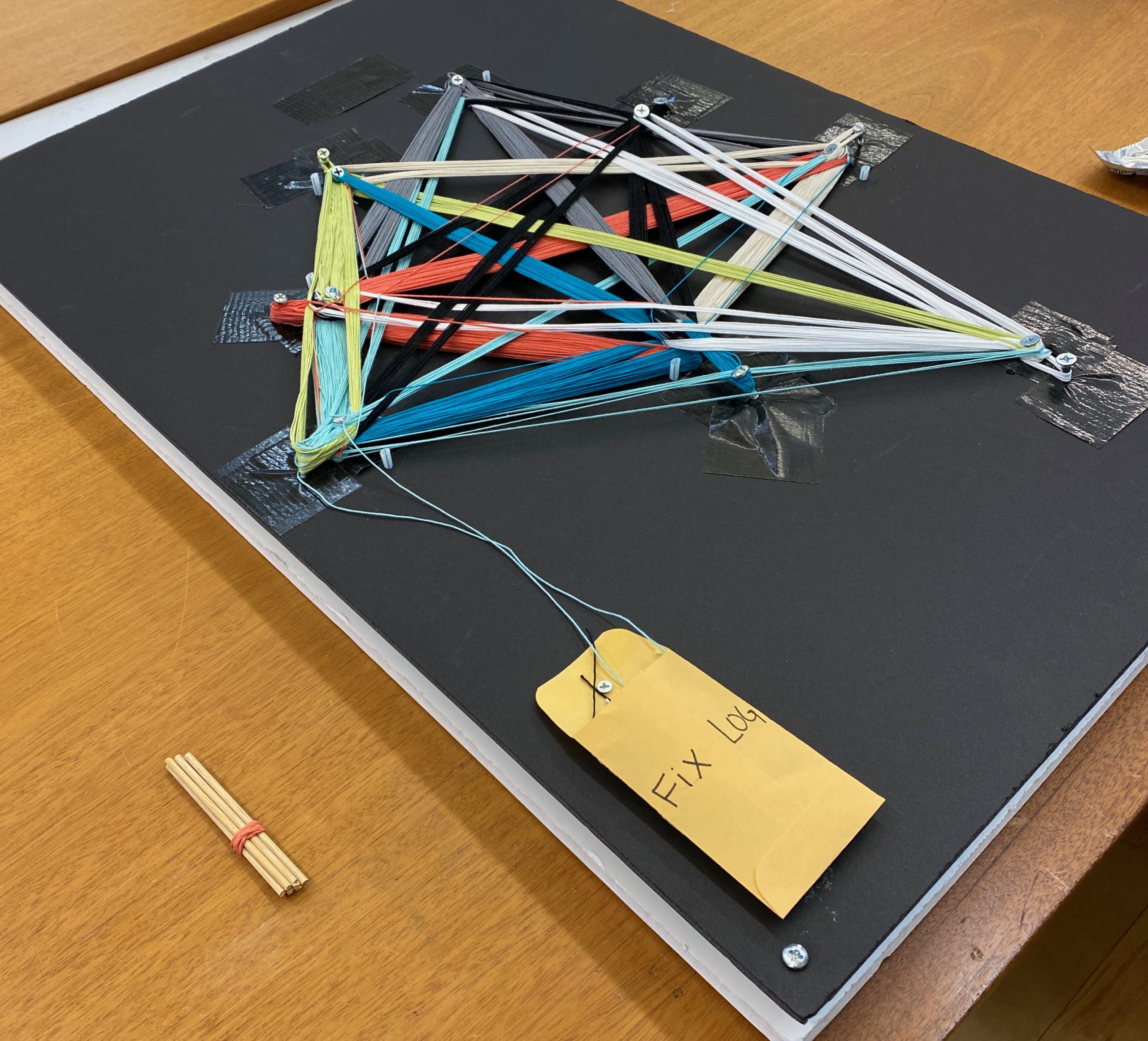
Individual Physicalization Process

Materials:

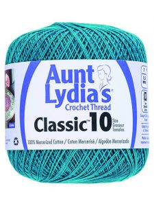
  • Thread (Aunt Lydia’s Crochet Thread Classic 10) – 8 different colors


  • Screws (various sizes) + Screw driver
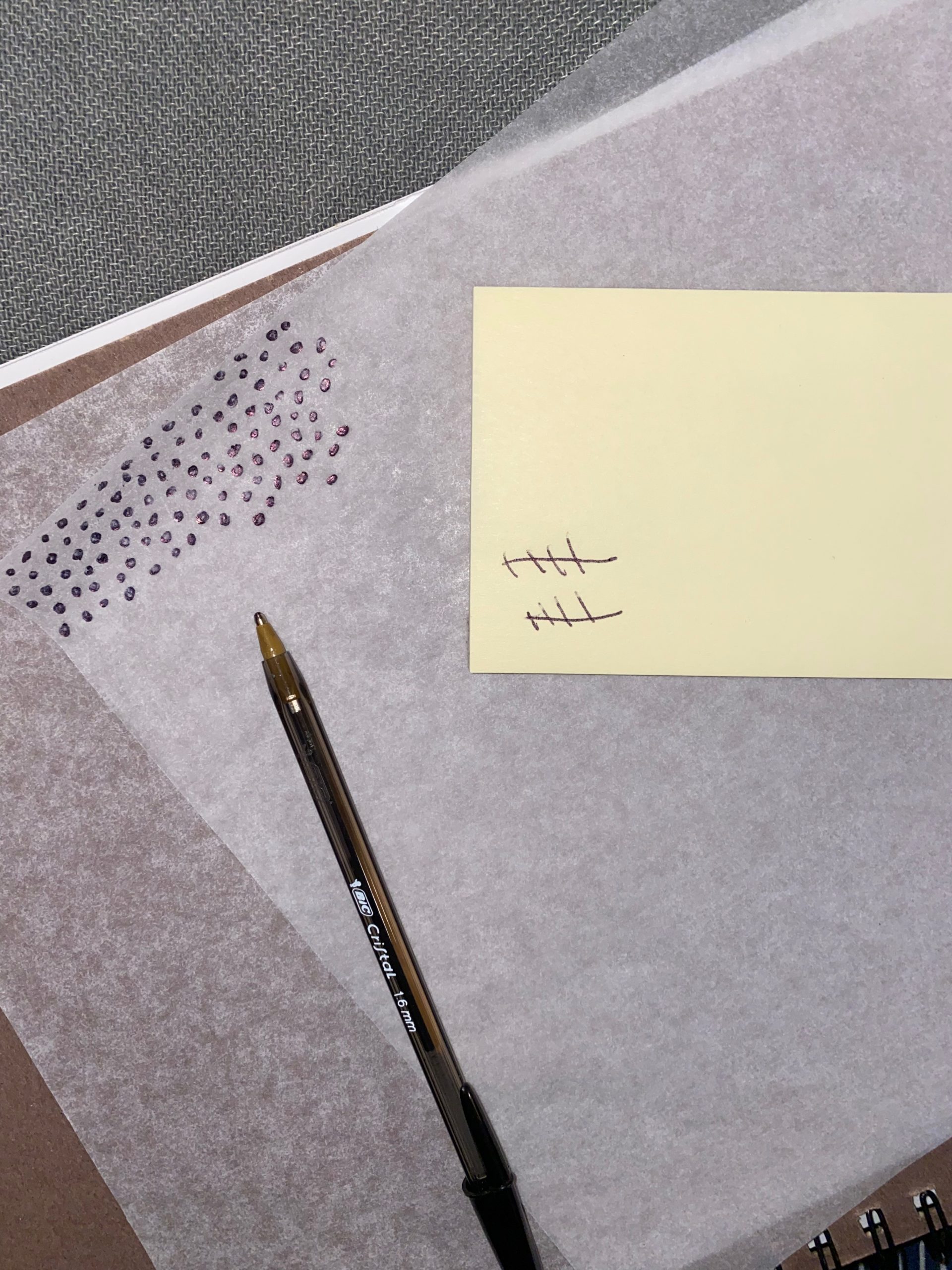
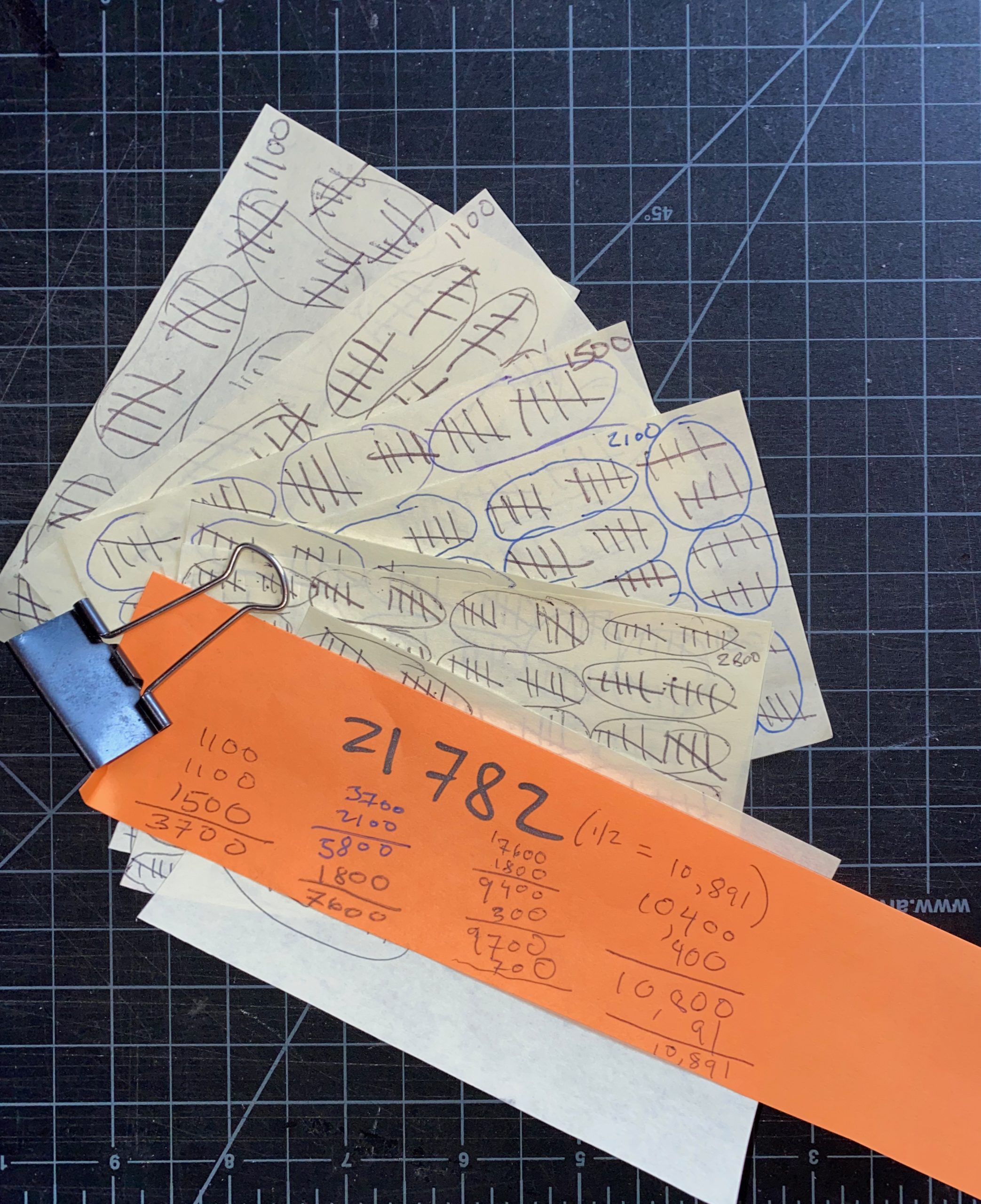
  • Tracing paper + pens
  • Spray adhesive
  • Drinking straws (regular and hard plastic versions)
  • Utility + exacto knife
  • Duct tape

Make the “Absence”

To represent the data what was not included from the dataset (21,782 rows), I created a textural layer that would be glued to the underside of the physical network graph’s board substrate. Using tracing paper (or any thin paper will do), I created dots with a regular ball point pen. The key to this process is to press down VERY hard when making the dots so that the thin tracing paper is embossed from pressure of the pen tip.

10,891 dots were created. I assigned each dot the value of 2 data points, bringing to overall total to 21,782 representative data points.

I used spray adhesive to attach all the dotted tracing paper sheets to the underside of the foam core board used for the network graph.

Make the Physical Network Graph:

Using the thinner foam core board, I laid out the labels of where the top 8 artist nodes would reside (using the Gephi output as a guide). I then assigned a color thread to each artist. I screwed in a screw for each node and wrapped the thread around 2 nodes, which created the edge. The nodes and edge tables with weight (occurrences) served as the “directions” to build the density of the edges between the nodes. Since space was limited, I assigned 2 occurrences for each loop connecting the 2 nodes. 

I didn’t anticipate the wrapping would be so thick, which in turn put a lot of stress on the screws, so I needed to reinforce the screw holes with duct tape.

Once the wrapping was complete, I installed the recording devices to the other foam core board. I recorded the name of each of the top 8 artists into each of the devices.

The board with the network graph was fastened on top of the sound device board with additional screws at each corner with a hard plastic straw section to serve as a shunt for extra support.

A hole was poked directly near each node where another straw section would be fed through to create a portal for a wooden dowel to pass through to engage the button on the sound device to replay the record name of  the artist.

Reflections

Making big data small doesn’t always translate, but the process provided the learning and experiencing through the process. Stark stated “interfaces that make data sets viscerally engaging could result in a more holistic process of individual decision-making, grounded in both our thoughts and our feelings”(Stark, 2014), which I can attest to personally. Which is also an interesting thought to consider- this process, this experience was definitely my own, but what about others?

Throughout the process I was painfully and frustratingly aware of the rigidity of the physical  domain – take digital for granted and can easily ignore what doesn’t “fit”. I came face to face with my bias by practicality. I ultimately had to make choices along the way to make a physicalization possible with the materials at hand. Do data scientists or other digital humanists make these types of concessions to realize a project goal? How many micro choices does it take to shift an analysis or arrival to a conclusion. 

felt when working with the data (frustration, elation, wonderment, curiosity, etc). It was certainly an indelible experience that will carry over into my future data work. There is a reorientation and respect to data processing as a result from this project. As Tim Schoof mentions in his article, The Future of Data Science Includes Slow Data Science, … “to represent data is that it really allows you to slow down and experience the data in real time. It is as much about the process, the experience, as it is about the end product” (Schoof, 2022).

-Jessika Davis

Additional documentation and Python scripts can be found within this GitHub Repository.